 Unbounded Labs
Bartholomew: A Vintage LLM
Cost to make$0.00
"The farther backward you can look, the farther forward you are likely to see." — Winston Churchill
We can't fully grasp modern questions like the rise of artificial intelligence, economic disruption, or automation while standing in the middle of them. Sometimes our best path forward is the one that takes us backward. In the past year, many have begun to explore this idea by applying it to large language models (LLM's). What can we learn about today's modern technology when we fuse it with information hundreds of years old? Recent models such as Talkie,Radford, Levine and Duvenaud. talkie — a 13B model trained on 260B tokens of pre-1931 English. talkie-lm/talkie-1930-13b-base and GPT-1900,Hla, M. GPT-1900 — a 3.3B model trained from scratch on pre-1900 text, to see whether it could arrive at quantum mechanics and relativity. michaelhla/gpt1900 have demonstrated that stripping away modern hindsight transforms an artificial mind from a simple archive into a powerful diagnostic lens. But while these models offer a proof of concept, true historical reasoning—like devising the transistor 20 years ahead of schedule—is still unreached. Material results remain the holy grail of historical AI. The next step, then, is to push historical LLM's into the future: state-of-the-art architectures, cleaner, more refined corpora, period-appropriate evaluations, and vintage-adapted post-training techniques. In this article, we introduce Bartholomew III, or Bartholomew for short, our attempt to move the needle of historical language modeling.
#Results
Bartholomew is a depth-32, 2.82B-parameter decoder-only transformer trained on 20.1B tokens of pre-1931 English. Every score below is Vintage CORE — CORE with its post-1930 knowledge removed, described under Evaluation — on the twenty tasks common to all three bundles.
Eval data from all 5 models on all Vintage Core
Every task in the common-20 intersection, grouped by domain. Scores are CORE's
centered accuracy — (accuracy − random) / (1 − random) — so 0 is chance and a
negative number means the model did worse than guessing.
Original
| Benchmark | Bartholomew | Bartholomew d24 | GPT-1900 d34 | Talkie 1930 13B | Modern d24 |
|---|---|---|---|---|---|
| Language modeling | |||||
| LAMBADA | 0.414 | 0.353 | 0.397 | 0.607 | 0.427 |
| Reading comprehension | |||||
| SQuAD | 0.203 | 0.114 | 0.127 | 0.553 | 0.354 |
| CoQA | 0.266 | 0.166 | 0.218 | 0.431 | 0.255 |
| BoolQ | -0.060 | -0.061 | -0.399 | 0.281 | -0.092 |
| Commonsense | |||||
| HellaSwag zero-shot | 0.166 | 0.098 | 0.124 | 0.356 | 0.356 |
| HellaSwag | 0.171 | 0.105 | 0.124 | 0.388 | 0.357 |
| CommonsenseQA | 0.086 | 0.134 | 0.053 | 0.075 | 0.147 |
| COPA | 0.360 | 0.220 | 0.180 | 0.460 | 0.340 |
| PIQA | 0.208 | 0.161 | 0.162 | 0.366 | 0.428 |
| Reference knowledge | |||||
| Jeopardy | 0.033 | 0.004 | 0.033 | 0.333 | 0.193 |
| BIG-bench Wikidata QA | 0.317 | 0.252 | 0.287 | 0.481 | 0.511 |
| BIG-bench language ID | 0.177 | 0.183 | 0.183 | 0.179 | 0.174 |
| Academic QA | |||||
| ARC Easy | 0.278 | 0.223 | 0.217 | 0.483 | 0.570 |
| ARC Challenge | 0.025 | -0.014 | 0.001 | 0.182 | 0.181 |
| OpenBookQA | 0.045 | 0.011 | 0.040 | 0.120 | 0.200 |
| LSAT analytical reasoning | 0.087 | 0.076 | 0.082 | 0.065 | 0.130 |
| Coreference | |||||
| Winograd | 0.297 | 0.341 | 0.392 | 0.641 | 0.421 |
| WinoGrande | 0.066 | -0.012 | 0.080 | 0.280 | 0.133 |
| Symbolic reasoning | |||||
| BIG-bench operators | 0.129 | 0.114 | 0.129 | 0.243 | 0.171 |
| BIG-bench repeat/copy logic | 0.000 | 0.000 | 0.000 | 0.062 | 0.000 |
Filtered
| Benchmark | Bartholomew | Bartholomew d24 | GPT-1900 d34 | Talkie 1930 13B | Modern d24 |
|---|---|---|---|---|---|
| Language modeling | |||||
| LAMBADA | 0.415 | 0.352 | 0.401 | 0.611 | 0.425 |
| Reading comprehension | |||||
| SQuAD | 0.213 | 0.119 | 0.139 | 0.542 | 0.348 |
| CoQA | 0.282 | 0.178 | 0.236 | 0.429 | 0.238 |
| BoolQ | -0.078 | -0.012 | -0.467 | 0.262 | -0.177 |
| Commonsense | |||||
| HellaSwag zero-shot | 0.188 | 0.115 | 0.144 | 0.384 | 0.354 |
| HellaSwag | 0.196 | 0.129 | 0.148 | 0.416 | 0.357 |
| CommonsenseQA | 0.061 | 0.126 | 0.050 | 0.065 | 0.155 |
| COPA | 0.380 | 0.240 | 0.160 | 0.500 | 0.340 |
| PIQA | 0.277 | 0.230 | 0.193 | 0.427 | 0.422 |
| Reference knowledge | |||||
| Jeopardy | 0.042 | 0.005 | 0.048 | 0.398 | 0.190 |
| BIG-bench Wikidata QA | 0.408 | 0.331 | 0.379 | 0.616 | 0.562 |
| BIG-bench language ID | 0.168 | 0.172 | 0.177 | 0.175 | 0.177 |
| Academic QA | |||||
| ARC Easy | 0.326 | 0.244 | 0.247 | 0.543 | 0.571 |
| ARC Challenge | 0.042 | -0.001 | 0.010 | 0.225 | 0.184 |
| OpenBookQA | 0.069 | 0.035 | 0.061 | 0.157 | 0.229 |
| LSAT analytical reasoning | 0.011 | 0.011 | 0.011 | -0.005 | 0.103 |
| Coreference | |||||
| Winograd | 0.282 | 0.333 | 0.385 | 0.626 | 0.436 |
| WinoGrande | 0.091 | -0.006 | 0.097 | 0.307 | 0.143 |
| Symbolic reasoning | |||||
| BIG-bench operators | 0.129 | 0.114 | 0.129 | 0.243 | 0.171 |
| BIG-bench repeat/copy logic | 0.000 | 0.000 | 0.000 | 0.062 | 0.000 |
Restyled
| Benchmark | Bartholomew | Bartholomew d24 | GPT-1900 d34 | Talkie 1930 13B | Modern d24 |
|---|---|---|---|---|---|
| Language modeling | |||||
| LAMBADA | 0.414 | 0.353 | 0.401 | 0.611 | 0.426 |
| Reading comprehension | |||||
| SQuAD | 0.205 | 0.110 | 0.137 | 0.532 | 0.344 |
| CoQA | 0.273 | 0.173 | 0.233 | 0.416 | 0.234 |
| BoolQ | -0.065 | -0.038 | -0.480 | 0.281 | -0.161 |
| Commonsense | |||||
| HellaSwag zero-shot | 0.188 | 0.118 | 0.150 | 0.373 | 0.344 |
| HellaSwag | 0.196 | 0.130 | 0.151 | 0.397 | 0.336 |
| CommonsenseQA | 0.068 | 0.138 | 0.047 | 0.067 | 0.152 |
| COPA | 0.360 | 0.240 | 0.240 | 0.440 | 0.320 |
| PIQA | 0.252 | 0.228 | 0.201 | 0.424 | 0.401 |
| Reference knowledge | |||||
| Jeopardy | 0.046 | 0.007 | 0.051 | 0.385 | 0.190 |
| BIG-bench Wikidata QA | 0.408 | 0.331 | 0.379 | 0.616 | 0.562 |
| BIG-bench language ID | 0.168 | 0.172 | 0.177 | 0.175 | 0.177 |
| Academic QA | |||||
| ARC Easy | 0.331 | 0.246 | 0.250 | 0.520 | 0.538 |
| ARC Challenge | 0.066 | -0.001 | 0.018 | 0.237 | 0.180 |
| OpenBookQA | 0.072 | 0.077 | 0.072 | 0.131 | 0.221 |
| LSAT analytical reasoning | 0.011 | 0.011 | 0.011 | -0.005 | 0.103 |
| Coreference | |||||
| Winograd | 0.311 | 0.282 | 0.458 | 0.641 | 0.407 |
| WinoGrande | 0.084 | 0.047 | 0.118 | 0.288 | 0.118 |
| Symbolic reasoning | |||||
| BIG-bench operators | 0.129 | 0.114 | 0.129 | 0.243 | 0.171 |
| BIG-bench repeat/copy logic | 0.000 | 0.000 | 0.031 | 0.062 | 0.000 |
#Leakage
The dataset is an independent reconstruction of the HISTORY-EVENT benchmark described in Pretraining Language Models on Historical Text.arXiv:2606.02991. This is not the authors' official dataset; our public reconstruction is at jbduran/history-event-reconstruction. We can see an increase after the knowledge cutoff starting around the 1900s for vintage models. In contrast, SmolLM3 (modern) remains broadly flat across decades, consistent with modern-event exposure.
#Pretraining
Arguably, the most important part of a model is its dataset. Curating a high-quality dataset means obtaining raw pre-1930s text that's clean, correctly dated, and large enough to pretrain on. Combining these constraints leads to significant challenges.
Of the three, we felt that text-cleanliness was the limiting factor in dataset curation and therefore was a natural place to begin. Optical character recognition (OCR) quality is a score representing how accurately text is captured from real-world images and scans. This is important because pretty much all text used in a historical model will have been sourced via OCR. Here is an example of poor OCR:
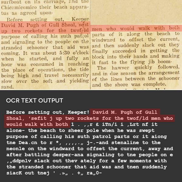
For us, OCR quality is measured as a per-document confidence score. Low-scoring documents carry systematic transcription errors and stray page furniture that, if left in, corrupt the corpus at the subword level: the tokenizer allocates vocabulary to garbage merges, and the model spends capacity modeling scanner noise instead of language. One possible way of mitigating OCR issues would be to re-OCR pre-1930s texts via a modern LLM-based OCR, but after considering this approach we found that it would cost too much. Assuming roughly 16–20 million pages for an 8–10B token dataset at around 500 tokens per page, re-OCRing even a small dataset would cost about $16,000 at Mistral OCR batch pricing.Mistral AI. Introducing Mistral OCR 3 — a vision-language OCR model with a batch API discount. mistral.ai/news/mistral-ocr-3
Alternatively, we found it best to source pre-existing datasets and transform the existing corpora. A few options stood out. Project Gutenberg is a high-quality dataset but is also very small.gutenberg.org — 75,000+ hand-proofread public-domain books. The American Stories dataset had great size, but we were concerned with the OCR quality due to the difficulty of OCR-ing newspapers.Dell et al. American Stories: A Large-Scale Structured Text Dataset of Historical U.S. Newspapers, NeurIPS 2023. arXiv:2308.12477 · dell-research-harvard/AmericanStories We kept searching, and came across Institutional Books 1.0. This dataset is a result of the digitization and post-processing work of the Harvard Library, boasting 242B tokens and almost a million documents.Cargnelutti et al. Institutional Books 1.0: A 242B Token Dataset from Harvard Library's Collections, 2025. arXiv:2506.08300 · institutional/institutional-books-1.0
Working from the Institutional Books (IB) dataset, we applied an aggressive OCR score threshold of 0.90, drawing on both OCRoscope and the OCR score from Google Books metadata, and required that the two metrics agree within 0.10 on any given document. Furthermore, we filtered by date (any undated books are rejected), we filtered for English (this resulted in the most rejects), and we filtered text with tokenizability scores less than 95 — a score indicating how efficiently a tokenizer encodes the text. This trimmed the 242B tokens down to 27B. We then deduplicated by book barcodes and shuffled the dataset. The result was our first cleaned dataset — bartholomew-dataset-v1.
Another phase of filtering targeted boilerplate text and OCR corruption that snuck through IB's filters. This consisted of removing useless headers, footers and library stamps, alongside gibberish symbols and antiquated characters through heuristic regex filters. We also followed Michael Hla's log-prior filter, which estimates a text sequence's unconditional log-prior probability by summing token-level log probabilities and then trims improbable or out-of-distribution tokens.Documents whose log prior falls outside the 2.5th–97.5th percentile band are dropped, trimming both ends of the distribution. See michaelhla/gpt1900. This phase resulted in bartholomew-dataset-v2. While we expected major improvements in our validation bpb (see Evaluation), our models actually saw a decline in performance because this phase removed most of the easy items for a model to replicate — that is, the boilerplate.
For our final phase, we decided to focus on the time period. Although we did filter previous stages by date, leaks and bad labeling would inevitably allow modern documents to contaminate our vintage dataset. We once again filtered through the boilerplate of documents, focusing on removing missed footers. However, the biggest part of this phase was the regex anachronism filter. We used a tiered banned words list to flag documents and remove them on too many "hits."
Rather than trimming, we removed entire documents when conditions were met. A single Tier 1 hit was enough to discard a document, while Tier 2 words required two occurrences. Tier 3 words never triggered removal on their own — they only counted when accompanied by at least one Tier 2 hit. We used this strategy later in midtraining to keep all of our data as vintage as possible. With all of these strategies, we created bartholomew-dataset-v3 — our best vintage dataset yet.
#Architecture
Every successful model builds on a proven foundation and modifies it for its needs. When Qwen trained their first model family (Bai et al.),Bai et al. Qwen Technical Report, 2023. arXiv:2309.16609 they started from Llama's architecture. Kimi K2 started from DeepSeek-V3's MoE architecture.DeepSeek-AI. DeepSeek-V3 Technical Report, 2024. arXiv:2412.19437 We used Karpathy's Nanochat as a base since it's highly optimized and easily modifiable.karpathy/nanochat — an end-to-end LLM pipeline in a single readable codebase. Nanochat is an end-to-end LLM pipeline (extending from tokenization all the way to inference) built around a single complexity dial — "depth". Depth drives model scaling and is what we use to research the model at different sizes. We abbreviated it to "d#", where the number corresponds to the chosen depth (e.g., d12 or d24). Within the codebase is the actual GPT module: a decoder-only transformer with rotary embeddings, QK-norm, untied embedding/lm_head, ReLU² MLP, Group-Query Attention, and Flash Attention 3.Shah et al. FlashAttention-3: Fast and Accurate Attention with Asynchrony and Low-precision, 2024. arXiv:2407.08608
While we started with almost all of nanochat's hyperparameters, we wanted to verify that they were optimal for our vintage data. Through later experimentation, we tested countless different hyperparameters, most notably context size and the Muon optimizer's momentum.
#Evaluation
We knew where our data was coming from, and how it would be processed, but before we could train anything we needed to know how to gauge progress. Think about it: how exactly do you quantify a good vintage model?
Validation BPB is a way of seeing how good a model is at autocompleting a set-aside, unseen piece of the dataset. Validation BPB is a great metric for pretraining, but it is dataset-specific. Consequently, we're not able to compare against other vintage or modern LLMs.
So we reached for CORE, the benchmark suite nanochat reports for its GPT-2 speedruns.Li et al. DataComp-LM: In search of the next generation of training sets for language models, 2024. arXiv:2406.11794. CORE averages a centered score over 22 tasks: (accuracy − random) / (1 − random), so 0 is chance and 1 is perfect. CORE is dataset-independent, cheap, and comes with a known GPT-2 reference point. One problem: CORE assumes a modern world model. Its tasks ask about websites, post-1930 organizations, brands, later scientific discoveries, and contemporary sports. Is our model dumb, or is it just being asked modern-laced questions?
We remove two benchmarks that cannot be salvaged, filter post-1930s content, restore small tasks to size with reviewed replacements, and build a second bundle where the surviving prose is rewritten into the style of 1800–1930. The result is Vintage CORE, released as a versioned dataset alongside its evaluator. That gives three measurements:
- Original — CORE as published.
- Filtered — post-1930 knowledge removed. Original prose.
- Restyled — same as filtered except vintage prose.
Data — headline scores
| Model | Corpus | Depth | Training tokens | Original | Filtered | Restyled |
|---|---|---|---|---|---|---|
| Bartholomew | Pre-1931 | 32 | 20.1B | 0.163 | 0.175 | 0.176 |
| Bartholomew d24 | Pre-1931 | 24 | 8.76B | 0.123 | 0.136 | 0.137 |
| GPT-1900 d34 | Pre-1900 | 34 | 22B | 0.121 | 0.127 | 0.139 |
| Talkie 1930 13B | Pre-1931 | — | 260B | 0.329 | 0.349 | 0.342 |
| Modern d24 | Modern | 24 | 8.76B | 0.263 | 0.262 | 0.253 |
The same broad strategy appears in TypewriterLM's HellaSwag-1800: filter the temporally unfair items, then rewrite the survivors.Pretraining Language Models on Historical Text, 2026. arXiv:2606.02991 · typewriter.chat We apply it across a full 20-task suite rather than a single benchmark.
#Ablations
In our hopes to push the historical modeling space forward, we're including a short space here to document our exploration of the many mechanics and quirks of vintage language models. We explored model behavior through ablations (aka experiments). The goal of ablations was to run experiments at a small scale and get results we could confidently extrapolate to our Bartholomew model. We tracked most of our ablations on GitHub via Issues.Every ablation has an issue with its config, its W&B run, and its result: Bartholomew GitHub issues. Below we list some of the more interesting ablations that guided our model's trajectory. Every run behind them — 39 in all, with their tokenizers, checkpoints and evaluations — is archived in bartholomew-experiments. We hope this all helps you in your own development.
Briefly, we want to also emphasize the importance of two key development tools we used: Weights and Biases, and model configs. Weights and Biases is a diagnostic service that tracks all things regarding model training.wandb.ai — learning rate, FLOPs, even GPU wattage. Model configurations are simply JSON files that define model hyperparameters for each run. While often unspoken of in ML engineering, these two things are essential for scalable and easy experimentation.
#EXP007 · Variance testing
When testing on a small stand-in model, we found that CORE scores varied significantly, even for identical models, which, unfortunately, threw off our judgments of multiple previous experiments. A valuable reminder to not take anything for granted. While there is significant variation for CORE scores at the d12 scale, the amount of variation shown in EXP005 was unprecedented.
#EXP005 · Modern and vintage mixture
A simple test to explore just how much our performance depends on dataset quality. Even a small inclusion of the heavily-optimized ClimbMix dataset late into the training schema — the last 20% of train shards — saw an enormous CORE boost: 0.0673 → 0.1003. This confirmed a suspicion we had carried for some time: our model's dominant bottleneck was the absence of modern data, not the quality of the vintage data we had curated.
#EXP010 · Longer context length
Since the average pre-1930s document length is hundreds of times larger than that of modern pretrain corpora, increasing context length early in the training pipeline could benefit from these larger text sequences.This experiment had a flaw worth noting: it used full attention rather than sliding-window attention. Surprisingly, performance gains were merely cosmetic, and early tokens in the attention pattern showed minimal improvement in learned representation. The benefits still outweighed the costs, and we kept a 4096 context length.
#EXP012 · Tokenizer
Our wildly unique pretrain corpus led us to test nanochat's built-in tokenizer variables — specifically document_cap, max_characters, and where documents start. A few findings emerged: random sampling improved compression ~1%, pushing max_characters above 80M barely improved compression, and high byte-fallback rates pointed to remaining OCR dataset junk. Despite the diminishing returns, it was cheap to train our tokenizer on our full corpus.
#EXP014 · Autoresearch
Prior to running our final model we ran 100 autoresearch experiments with the goal of improving our val/bpb relative to our compute budget. We adapted Karpathy's autoresearch to our model.karpathy/autoresearch — an agent edits one training file, runs a five-minute experiment, reads validation BPB, and iterates. Each experiment runs on a single H100, and the harness we ran them through is open source as bartholomew-autoresearch. The training script runs for a fixed time budget of 5 minutes. GPT 5.6 Sol extra high was the model used for autoresearch and the loop ran for 10 hours. There were 26 improvements that reduced validation BPB from 1.244632 to 1.223533, or 1.70%. We only kept improvements to the Muon optimizer's momentum since they were the most impactful and we didn't have the time to scale up more potential improvements. A constant momentum of 0.90 was the best d12 result and was adopted for the final d32 run.
Nanochat's original architecture is already very optimized, and much of the low-hanging fruit has already been eaten. Many of the improvements from autoresearch were not novel. The models clearly understand the objects they manipulate at a deep level, and yet very few genuinely new ideas emerge, which makes it hard to tell if this is an artifact of the speedrun setup or a real capability of the agent models.
#Midtraining
Midtraining sits between pretraining and downstream use: instead of continuing on the same broad corpus, we shift the data mixture toward a smaller, higher-quality set of documents while decaying the learning rate. The goal is to spend the model's final optimization steps on the text we most want it to internalize, which for us meant pre-1930s math, science, technology, and medicine. This section covers both how we built the midtraining dataset, and how we scheduled the run itself.
For our midtraining dataset, we focused on finding high-quality math, science, technology and medicine documents from before the 1930s. For clarity, we broke each major step into stages. We started out by extracting these documents using their subject tags from bartholomew-dataset-v1. Then, we extracted vintage documents from the Internet Archive by filtering by topic for Math, Science, Medicine, and Technology documents using their published date. We then de-duped these documents and used an OCR filter of 0.85. To get a second opinion, we filtered out 10% of documents using additional OCR filtering with OCRoscope (0.85) and an alphanumeric ratio of 0.65. Due to math documents having many different symbols, we wanted to keep the alphanumeric ratio relatively relaxed. Then, we filtered for OCR artifacts and removed portions of the boilerplate off of documents (headers, library stamps, etc). We mimicked our filtering in our main corpus using a log prior filter (2.5, 97.5).
Finally, we made sure our midtrain dataset was as vintage as possible, running it through the footer filter and the banned words list. As we cleaned our original corpus, we learned valuable tools and methodology for dataset cleaning. We applied this knowledge to midtraining extensively. After all the cleaning in midtraining, we removed 24% of the original midtraining data, leaving us with 608M tokens of high-quality midtraining data — bartholomew-midtrain.
For the midtraining itself, we mimicked Hugging Face's SmolLM with midtraining in stages of decay.SmolLM's recipe decays the learning rate in stages while progressively raising the share of high-quality data. huggingface.co/blog/smollm3 Training ran in three stages. Because midtrain documents are much shorter than bartholomew-dataset-v3 documents, we used tokens rather than documents to measure the mixtures of midtrain to original corpus. We wanted our midtrain data to have less than 3 epochs, so we used that as a guide for the ratios at each stage.
For a learning rate scheduler, we used nanochat's Warmup-Stable-Decay (WSD) starting decay at around ~35%. On the other hand, SmolLM started decaying at around ~75%.
One of the biggest pitfalls on this journey was during our final model run. We assumed that the size of midtrain documents would be roughly smaller than the original corpus. We were right, but we didn't realize how drastically smaller these midtrain documents were. Since we used document count rather than tokens to create the mixtures used for midtraining, we had to recreate our datasets with ratios with tokens rather than document counts. Since our final model was already running when we discovered this bug, we had 36 hours to create these new mixtures before our model would need them. Ultimately, we were able to get the mixtures ready for the model in time along with learning a valuable lesson — verify your intuition.
#Midtraining results
The goal of midtraining was to use the model's final optimization steps to internalize a smaller, higher-quality body of text. While we hoped this targeted phase would produce clear improvements, our evaluations do not provide conclusive evidence that midtraining was beneficial.
In contrast to these results, there is no conclusive evidence that our midtraining dataset is harmful. In fact, we did see a slight increase on the standard CORE scores (0.1369 to 0.1402). Although this is promising, it is not a statistically significant increase. Due to the lack of resources and time, we were not able to run ablations on different data mixtures for midtraining. Because of this, we had to rely on a meager number of experiments before scaling up our model.
#Scaling
Scaling up to the d32, we knew we needed a hardware upgrade. Previously, we were using A100s with Flash Attention 2 for all experiments. We set our eyes on H100s for their 2–3 times speed up with Flash Attention 3. After researching multiple different options for leasing, Vast.ai was by far the most price efficient.vast.ai — a marketplace for spot GPU rental, priced per host rather than per region. We considered running a 4x or 8x cluster to speed up the runs. Preparing for the 4x and 8x clusters, we created a Docker image that has all of our dependencies and saves us 30 minutes on setup. We ran our first d24 on a 4x cluster to test the new Docker image. It finished in 5.5 hours and cost about $34. One difficulty in using a multi-GPU cluster is that resuming requires similar hardware unless you are willing to drop the momentum of the optimizer, losing around 20 steps of learning. While there are possible solutions to circumvent this problem, we decided to resume our runs on the same hardware to spend our time in more valuable areas.
Compared to other options for leasing, Vast.ai's GPUs shined brightest when using single devices. Since there are far more options to select from for single devices, it was far easier to find a bargain — especially past 11pm EST. While typical H100s cost ~$2–3 an hour, we were able to snag one for 99 cents an hour. Starting the d32 run Friday morning and with our budget approaching its maximum, we decided to opt for the single H100 as speed was not a huge priority. The run took 5 days on a single H100 and cost about $140. Throughout our run we held a 60 MFU on our H100. Our loss had minimal spikes, and throughput held at a consistent 50k tokens per second. We had to pause the run at step 5500 (57%) to fix the midtraining shards. This resulted in 1 hour and 30 minutes of downtime. The run remained healthy throughout, and the full d32 run is public on Weights & Biases, as are the two d24 runs that preceded it.The d24 ran in two parts on the 4x cluster: e69c1e59 · 2fa1b744
#Post-training
Making our model "feel" and act like an individual from the 1930s falls under the category of supervised fine-tuning. SFT datasets are abundant for normal models, but for models trained exclusively on pre-1930s data the vast range of options vanishes.A few do exist — vintage-ft-v2 and Violet-sft among them — but none at the scale or specificity we needed. Because authenticity was a priority for us, it seemed smart to start by sourcing authentic question and answer (q/a) content that's already available online from the time period. This led to catechisms — texts specifically written in a question and answer format. About thirty catechisms total were sourced with topics such as engineering, logic, music, world history, and philosophy. A thorough extraction process included filtering, cleaning, enriching, and joining the q/a pairs. About 12k rows (with ~25% being multiturn conversations) were collected (authentic-pre1930-sft). For comparison, Hla's GPT-1900 model was trained on roughly 50k rows.Vintage-exam-qa. See michaelhla/gpt1900.
Research suggests that more important than size is quality and diversity.Zhou et al. LIMA: Less Is More for Alignment, 2023. arXiv:2305.11206 Since authentic sources would never be able to cover the many types of behaviors we wanted our model to exhibit, we pivoted to generating q/a pairs instead. Inspired by TypeWriterLM's History-SelfInstruct pipeline, we opted for grounded-answer based generation. In essence, pull excerpts from our corpus, trim and shape them to make good answers, and then generate a feasible question based on the given answer. This means generation and anachronism are halved; only the questions can carry an anachronistic risk. Further, because models typically mask the questions when fine-tuning, in theory, the model never updates its weights directly on anachronistic text (though context still picks it up). To encourage diversity, about ten categories of q/a pairs were drafted consisting of narrative generation, knowledge recall, opinions, STEM reasoning, refusal calibration, etc.
Total counts per question category
synthetic-pre1930-sft · 416k rows, ~70M tokens
Data
| Group | Rows |
|---|---|
| multiturn_qa | 131.8K |
| knowledge_qa | 65.9K |
| composition_qa | 40.7K |
| opinion_qa | 38.6K |
| narrative_grounded | 38K |
| narrative_fiction | 31.7K |
| reasoning_qa | 24.1K |
| verse_qa | 17.4K |
| how_to_qa | 17K |
| stem_reasoning | 8.3K |
| calibration_qa | 2.7K |
Excerpts were algorithmically cherry-picked from the corpus, and then prompts were refined for each category to avoid context-bare, irrelevant questions, and phrase-repetition.
Examples of bare questions:
- "What error does the writer discover in the note from the Insurance Society concerning the premium?" — references the passage's author and an unnamed note; unanswerable to anyone who didn't read it.
- "What was the nationality and age of the captain of the corsair?" — which corsair?
Questions after tuning the prompt:
- "What was the method of cure, as given in 1857, for the disease in cattle evidenced by a frequent slight kicking of the hind foot?"
- "…the steamer built by Workman & Clark, of Belfast, which possessed a greater carrying capacity than…"
The result is synthetic-pre1930-sft, a monstrous 416k-row (~70M tokens) dataset consisting of about 33% multiturn conversations, and roughly half of the whole dataset purely knowledge-based q/a pairs. The remaining half consists of the less common question types meant to encourage diverse behavior and reduce hallucinations. Two highlights: STEM reasoning, a modestly sized intellectual reasoning set, and refusal calibration, a vital non-answer set fostering honesty. Pairs are categorized, dated, and graded, making this highly adaptable to different cutoff dates, SFT curriculums, and model personalities.
Grading is designed to answer the question, "How well does the q/a pair teach the model the intended goal of its category?" As shown in Figure 21, grading dramatically changes the landscape of the dataset. Around 196k q/a pairs are graded ≥ 95, and this increases to roughly 297k (+100.6k) for pairs ≥ 90. Grading is subtractive: if the model finds defects in the q/a pair, then the pair loses points. Differences in scores above 95 can, therefore, reasonably be reduced to noise. As such, we found that questions graded below 80 were not worth including in our final fine-tuning spread.
Speaking of fine-tuning spreads: Chen et al. and Kaur et al. demonstrate that a small, rich dataset consistently outperforms a much larger, noisy one.Chen et al. AlpaGasus: Training a Better Alpaca with Fewer Data, 2023. arXiv:2307.08701 · Kaur et al. Instruct-SkillMix, 2024. arXiv:2408.14774 Applying these insights to our dataset means that we shouldn't naively dump all of the q/a pairs into our model. A fine-tuning "curriculum" — as in a specific spread of learning material — needed to be concocted that would suit our model best. Six curricula were created to explore different ways of distributing the data. We wanted to find what drove the best model performance: data quantity, data quality, token distribution, domain scheduling, or domain difficulty. Surprisingly, we found that perhaps less isn't more in our case: our model chatted significantly better on the largest quantity of data. A cumulative 362k rows (~75M tokens) across 3 stages, progressing from easier to harder questions, thresholded at grades above 80, led to the best chatting experience by far. The 362k training rows were even later pushed to ~650k in a further iteration.
How does one build a canoe?
#Dataset limitations
Right at the end of the project, significant limitations surfaced regarding our fine-tuning coverage. Experimentation on the smaller d24 model displayed weird quirks. For example, the model could handle questions just fine, but ask the very same question without a question mark and the model would collapse down to its base model behavior, spewing hundreds of incoherent tokens and often degrading into repetition. Similarly, the model couldn't handle unparseable text, typos, or simple conversational openers such as "Hello", or "How are you?". These types of inputs weren't included in the fine-tuning dataset, so the model had no register for them.
The final d32 (2.8B) model appeared to generalize much better and was able to handle out-of-distribution inputs well. Still, the issues persisted and it led to a few last minute techniques being applied. One solution was to introduce artificial noise into the existing SFT corpus. Periodically and deterministically removing words, transposing letters, and adding or removing capital letters, punctuation, and spacing from questions made the model more sturdy at inference.
Larger-scale input corruption and diversity still needed to be addressed, though. So, a second solution was to create a complementary dataset aimed at teaching the model to respond as intended to outlying data. We made Robust-SFT for this purpose. User input that was uninterpretable, such as heavy typos, gibberish, or completely random character strings were paired with corpus-verbatim non-answers, such as "I beg your pardon" or "That is beyond me". 2,000 rows were synthesized across 11 classes of input corruption. Around 200 period and era grounding q/a pairs were synthesized to give the model some stiffness in this area. This comes with the highest anachronism risk, however, as they aren't corpus-grounded. Additionally, two types of conversational data were added: one which handled confusing but grammatically correct statements, and another prioritizing multiturn conversations and exchanges, which was very rare in the original dataset. 7,338 rows total, distributed across each stage of the original SFT dataset.
Despite our efforts, the issues weren’t completely fixed. Normal, structurally correct input without punctuation was still very volatile (pointing to an undertrained and underrepresentative fine-tuning). With time running low, we couldn’t spend more time curating data for the model to train on. We had to include a hotfix. The simplest change was to artificially append punctuation to the end of the user’s input. When experimenting, this cut the deterioration rates in half. Even better, though, was to prime the chat by prepending one full conversation turn. It’s like system prompting but simpler. The model essentially has the context of an earlier pre-specified introduction that the user doesn’t see. Our model is sufficiently trained on multiturn conversations, so it “recognizes” every interaction and responds properly even to those without proper grammar. The model that came out of all this — the C3 curriculum plus the robustness rows, branched from the base d32 at step 9,600 — is bartholomew-sft, and it is what the demo serves.
#Evaluations
ChatCOREnanochat's chat evaluation: scripts/chat_eval.py · tasks/ is another benchmark suite reserved by Karpathy for models that come through the nanochat pipeline. The synthetic-pre1930-sft dataset was created with ChatCORE in mind. Unfortunately, evaluations on this benchmark weren’t run during development. It turns out that ChatCORE is quite a biased benchmark and is mostly in place just to see how well a model learns Karpathy’s built-in fine-tuning tasks. In fact, ChatCORE is the reserved, set-aside validation set of nanochat’s fine-tuning tasks. So when we don’t fine-tune our model on his examples, the model does… poorly:
Because of the ChatCORE oversight, Bartholomew's post-training remains largely unevaluated.
#Hosting
With training finished, we needed somewhere to run inference. Our budget could not cover an always-on GPU, so we looked only at serverless providers, comparing Modal, RunPod, and Beam along with a few smaller options. Beam won initially on paper: $30 in free credits and an advertised RTX 4090 at $0.69 per hour.
In practice, Beam gave us trouble, and almost all of it showed up around cold boots. Every time we explicitly requested a 4090 we landed on an unhealthy worker. A10G requests were sometimes filled with physical 4090 hardware instead, and those 4090s ran fine. On release day, however, an A10G-requested container took 270 seconds to become ready, including 266 seconds just to read the model weights. Its replacement took another 138 seconds. Beam's edge also returned occasional 5xx responses while containers were starting, which a visitor experiences as a failed request rather than a slow one.
We switched production to Modal after testing six independent cold containers. Modal's cold starts ranged from 12 to 26 seconds, with a median of 13 seconds, while warm inference remained effectively instantaneous. Our deployment prefers an A10 but can fall back to an L4 or L40S when capacity is constrained. The model weights are stored in a cached image layer, the model loads before Modal accepts traffic, and GPU memory snapshots remain disabled because they are still experimental and do not improve storage-bound loading.
At Modal's current rates, our A10 configuration, including two CPU cores and 16 GiB of memory, costs approximately $1.32 per running hour, or about $0.22 for a full 10-minute warm period. With five to ten visitors arriving at widely separated times, we project roughly $8 to $16 in compute usage during the first week. Closely grouped visitors would share the same warm container and cost less.Modal pricing
We would not use Beam again for this workload. Modal has so far given us substantially faster and more consistent cold starts, although we are keeping the old Beam deployment available temporarily as a rollback target.
#Finances
Training a language model is constrained as much by compute costs as by technical considerations. For this project, we worked with the limitations of being students without external funding or institutional support. Despite these constraints, we were able to train and evaluate a model that we are proud of, while keeping our overall expenses relatively modest.
For our ablation experiments, our primary expense was Google Colab Pro, followed by compute rented through Vast.ai. The d24 and d32 cost about $34 and $140; the remaining Vast.ai spend covered two d12 runs, midtraining ablations, autoresearch, leakage and Vintage CORE evaluations, SFT, and ChatCORE. We used Hugging Face Pro for hosting our datasets and model checkpoints.
Claude Code subscriptions for the three of us ran for three months. Jonathan used Codex for three months to audit evaluations and run the autoresearch loop. Zach used DeepSeek to generate and grade the SFT dataset. OpenCode was used only to build Vintage CORE: we spent $15 across two subscriptions, while its dashboard estimated the equivalent raw API calls at about $74.
In total, our recorded expenses were approximately $757 before hosting. We spent $45 on Beam for the shadow release, and adding Modal's projected $8 to $16 for the first week puts the first-week total at roughly $810 to $818. This was not a fixed budget established at the beginning of the project; rather, it represents what we ultimately spent across development, training, and experimentation. The breakdown of these costs is shown below:
| Service | Cost |
|---|---|
| Vast.ai — GPU leasing | $227.18 |
| DeepSeek API | $174.93 |
| Google Colab | $70.00 |
| Claude Code | $180.00 |
| Codex | $60.00 |
| Hugging Face Pro | $30.00 |
| OpenCode | $15.00 |
| Beam hosting, shadow release | $45.00 |
| Modal, first-week projection | ~$8.00–$16.00 |
| Projected first-week total | ~$810.11–$818.11 |
#Conclusions
Our goal throughout this project was to determine how far careful data selection, training decisions, and limited compute could take a vintage language model. Exploring this niche field gave us insight into countless problems that the frontier labs do not experience, such as the lack of large amounts of high-quality SFT data. The results are not uniformly conclusive, but they give us a useful account of what worked, what did not, and — perhaps most importantly — what we would change in a future training run.
Looking back, there are several aspects of the training process that we would approach differently. During pretraining, we would have spent more time refining and validating the dataset before moving on to ablations. We also would have conducted a more thorough set of learning-rate experiments rather than relying primarily on established recommendations. For midtraining, we would have applied more aggressive filtering to the corpus, potentially using an LLM-based quality filter similar to the approach used by FineWeb-Edu. Additionally, budget and time constraints prevented us from systematically testing different mixtures of midtraining data, leaving an important part of the training recipe unexplored. Finally, delays in producing our final model compressed the timeline available for post-training, limiting the amount of time we could devote to refining the SFT dataset.
Despite these shortcomings, the process was an invaluable learning experience. Each limitation exposed a different challenge in training language models, from dataset construction and hyperparameter selection to experiment design and project management. While there are undoubtedly many things we would change in hindsight, these lessons provide a much stronger foundation for approaching our next training run.
Despite these challenges, we are proud of how much we accomplished over the summer while balancing the project with other commitments, including summer coursework. As researchers, we learned an enormous amount about training and evaluating language models, and we are especially proud of the resources we produced. bartholomew-dataset-v3 is one of the first open-source filtering efforts focused on Institutional Books textbooks, while Vintage CORE provides a valuable evaluation benchmark for future vintage models. Although our SFT dataset is not perfect, the work required to create it demonstrated just how challenging building specialized SFT datasets can be. Most importantly, we are proud of how we worked together through deadlines, problems, setbacks, and successes. We are proud of the model we produced and what we learned along the way. As the first project for our lab, we consider Bartholomew an enormous success and a valuable foundation for our future work.
#Acknowledgements
This project is built on work others did in the open.
- Andrej Karpathy — for nanochat, which this codebase forks, and autoresearch. His work has made from-scratch LLM training something a small team can actually carry end to end.karpathy/nanochat · karpathy/autoresearch
- Hugging Face Smol Models Research — for The Smol Training Playbook, the most useful practical guide to training a model from scratch that we found, and the closest thing the field has to an honest operations log.The Smol Training Playbook, by HuggingFaceTB.
- Talkie — the first vintage LLM we heard of, and the one that showed us the thing could be done at all.Introducing Talkie · talkie-lm/talkie-1930-13b-base
- Michael Hla — for the log-prior filter, which we adopted wholesale into our own cleaning cascade. There are many other great ideas he had that we wish we could explore further.michaelhla.com · Machina Mirabilis · michaelhla/gpt1900
- zakarth and croqaz — from the VintageLLM Discord, for advice and support throughout the creation of this model.zakarth · croqaz
#Citation
Please cite this work as:
Unbounded Labs, "Bartholomew: A Vintage LLM", Unbounded Labs Research, Aug 2026.Or use the BibTeX citation:
@article{unboundedlabs2026bartholomew,
title   = {Bartholomew: A Vintage LLM},
author  = {Unbounded Labs},
year    = {2026},
journal = {Unbounded Labs Research},
note    = {https://unboundedlabs.ai/blog/bartholomew}
}